Fitting bifurcation structure, not voltage traces: Reduced neuron models that preserve physiological parameter dependence

Reviewer #1 (Public review):

[Editors' note: this version has been assessed by the Reviewing Editor without further input from the original reviewers. The authors have addressed the comments raised in the previous round of review.]

Summary:

From a big picture viewpoint, this work aims to provide a method to fit parameters of reduced models for neural dynamics so that the resulting tuned model has a bifurcation diagram that matches that of a more complex, computationally expensive model. The matching of bifurcation diagrams ensures that the model dynamics agree on a region of parameter space, rather than just at specially tuned values, and that the models share properties such as qualitative features of their phase response curves, as the authors demonstrate. A notable point is the inclusion of extracellular potassium concentration dynamics into the reduced model - here, the quadratic integrate-and-fire model; this is straightforward but nonetheless useful for studying certain phenomena.

Strengths:

The paper demonstrates the method specifically on the fitting of the quadratic integrate-and-fire model, with potassium concentration dynamics included, to the Wang-Buzsaki model extended to include the potassium component. The method works very well overall in this instance. The resulting model is thoroughly compared with the original, in terms of bifurcation diagrams, production of various activity patterns, phase response curves, and associated phase-locking and synchronization properties.

Weaknesses:

It is important to note that the proposed method requires that a target bifurcation diagram be known. In practical terms, this means that the method may be well suited to fitting a reduced model to another, more complicated model, but is not likely to be useful for fitting the model to data.

Reviewer #2 (Public review):

Summary:

The authors derive an integrate-and-fire model to describe the dynamics of a more complex Wang-Buzsaki model and compare the two models. A detailed discussion of bifurcation schemes in both models is convincing and allows us to evaluate the simpler model.

Strengths:

The idea is interesting, and the mathematical approach appears to be convincing. In addition, differences between the simple and original models are also discussed.

Author response:

Public Reviews:

Reviewer #1 (Public review):

Summary:

From a big picture viewpoint, this work aims to provide a method to fit parameters of reduced models for neural dynamics so that the resulting tuned model has a bifurcation diagram that matches that of a more complex, computationally expensive model. The matching of bifurcation diagrams ensures that the model dynamics agree on a region of parameter space, rather than just at specially tuned values, and that the models share properties such as qualitative features of their phase response curves, as the authors demonstrate. A notable point is the inclusion of extracellular potassium concentration dynamics into the reduced model - here, the quadratic integrate-and-fire model; this is straightforward but nonetheless useful for studying certain phenomena.

Strengths:

The paper demonstrates the method specifically on the fitting of the quadratic integrateand-fire model, with potassium concentration dynamics included, to the Wang-Buzsaki model extended to include the potassium component. The method works very well overall in this instance. The resulting model is thoroughly compared with the original, in terms of bifurcation diagrams, production of various activity patterns, phase response curves, and associated phase-locking and synchronization properties.

Weaknesses:

It is important to note that the proposed method requires that a target bifurcation diagram be known. In practical terms, this means that the method may be well suited to fitting a reduced model to another, more complicated model, but is not likely to be useful for fitting the model to data. Certainly, the authors did not illustrate any such application. Secondly, the authors do not provide any sort of general algorithm but rather give a demonstration of a single example of fitting one specific reduced model to one specific conductance-based model.

We thank the reviewer for this critical assessment. It is true that we demonstrate our approach using as target the bifurcation diagram of a more realistic model. In principle, the method would be applicable to experimental systems if parameter space is sampled under appropriate experimental conditions, e.g., by recording at different extracellular potassium concentrations. However, this is challenging: generating reliable” experimental bifurcation diagrams” would require tightly controlled experimental repetitions under various conditions, particularly for reconstructing two-dimensional bifurcation diagrams. We hope that this work encourages the development of such methods. We have added a discussion of this point; see the paragraph starting at line 549.

We have also included a general algorithm (Table I) and provide a second example illustrating the procedure (Supplementary Fig. S2).

Finally, the main idea of the paper seems to me to be a natural descendant of the chain of reasoning, starting from Rinzel - continuing through Bertram; Golubitsky/Kaper/Josic; Izhikevich; and others - that a fundamental way to think about neuronal models, especially those involving bursting dynamics, is in terms of their bifurcation structure. According to this line of reasoning, two models are “the same” if they have the same bifurcation structure. Thus, it becomes natural to fit a reduced model to a more complicated model based on the bifurcation structure. The authors deserve credit for recognizing and implementing this step, and their work may be a useful example to the community. But the manuscript should have described and cited this chain of works to put the current study in the correct context.

We have added a paragraph in the Discussion section (starting at line 517) to better situate the manuscript within the relevant literature and to explicitly acknowledge the chain of work.

Reviewer #1 (Recommendations for the authors):

Please see my public review. In line with my comments, I recommend that the authors either (a) provide a general algorithm for fitting at least a class of reduced models (i.e., those that satisfy some general assumptions) to a class of bifurcation diagrams, or (b) provide at least one more example of implementing their method. Step (b) would not need to be done to the same degree of thoroughness as the example they provided (e.g., the PRCs and synchrony need not be considered), but to me, this step would be very important if (a) is impractical. Otherwise, the paper should probably be rewritten to de-emphasize the message that this is a general method; instead, this should be a paper about specifically fitting the QIF (with potassium dynamics) to the Wang-Buzsaki model (with potassium dynamics).

We provide a general algorithm for deriving a quadratic integrate-and-fire model with dependence on a biophysical parameter by fitting the bifurcation structure of a given class I conductance based neuron model near an SNL bifurcation induced by this parameter; see Table I.

In addition, we provide a second example of the reduction procedure: motivated by Hesse et al. (Nature Communications, 10.1038/s41467-022-31195-6, 2022), we derive a QIF model that captures dependence on temperature instead of potassium concentration; see Supplementary Fig. S2.

Not surprisingly, I also think it’s essential that the authors describe and cite the chain of works on thinking of neuronal models in equivalence classes based on bifurcation diagrams, and make clear that this paper builds on the ideas set forth in that chain.

We thank the reviewer for this comment. As mentioned above, we have added a paragraph in the Discussion section, starting at line 517, to acknowledge this chain of work.

Also, the authors should make clear that their method is not one for fitting a model directly to data, which will require rewriting at least the first paragraph of their Discussion section.

We thank the reviewer for helping us make our manuscript clearer. To avoid confusion, we have clarified this point already in the Introduction (see lines 52-57) and have included a new paragraph in the Discussion (starting at line 549).

Other specific corrections are:

(1) Typos should be fixed, as the paper has several. The first line of the abstract has one (“concentrations” → “concentration”), for starters. “Original model” on pg. 3 is missing “be” in “can defined”. “ceases” → “cease” on pg. 13. “nerons” → “neurons” on pg. 19. “standart” → “standard” pg. 24.

Done. Additional typos were also corrected.

(2) The abstract mentions “consequences in networks” in its second sentence. This is misleading because studying network dynamics is not at all the main emphasis of the paper, but rather a corollary application of the main ideas, so some restructuring of the abstract is needed. Similarly, the final abstract sentence overstates somewhat what was done with studying synchronization and should be rewritten more precisely.

We have restructured the abstract accordingly.

(3) For readers who are interested in the ideas here but not familiar with the QIF model, it will be very difficult to follow the first paragraph of Results. Elementary aspects of QIF dynamics should be explained here (e.g., what is the saddle-node bifurcation), and a basic figure panel about this should be included in Figure 1.

We added a supplementary figure (Figure S1) adapted from Izhikevich for readers who might not be familiar with the QIF model.

(4) Bottom lines of page 3 should be reworded to make clear that the slow variables are averaged over each member of a family of fast subsystem limit cycles. Also, “one limit action potential cycle” is an awkward phrase.

We rephrased this sentence (see paragraph starting at line 140).

(5) Text under system (1) – why isn’t c mentioned? Also, references to Figure 3 should be to Figure 2 here. And authors should state what they mean by “target model” and be clear about whether it includes potassium dynamics and/or pump current.

c scales the parabola corresponding to the branch of fixed points, given by c(I_app − I_SN,0 − I_pump) = −a(ν − ν_SN)². Consequently, it also affects the position of the homoclinic bifurcation: In the previous version of the manuscript, c was inadvertently omitted from the expression for the branch of fixed points; this has now been corrected. See paragraph starting at line 154.

Figure references have been corrected.

By target model, we mean the conductance-based model that includes potassium dynamics and a pump current, in our case System 4. We clarified this point at the beginning of the Results section (see paragraph starting at line 116). Throughout the manuscript, we now explicitly indicate when we refer only to its fast subsystem and whether the pump current is included. In particular, note that the parameter derivation shown in Figure 4 is performed on the fast subsystem of the target model, in the absence of the pump current. I_pump can be considered as a potassium-dependent contribution to the applied current, and can be added a posteriori to the QIF model. See paragraph starting at line 162.

(6) Next par: is the “saddle-node bifurcation” that with I_app as bifurcation parameter? Please clarify.

Yes, it is the saddle-node bifurcation with I_app as bifurcation parameter. We have clarified this in the manuscript; see the paragraph starting at line 170.

(7) Bottom pg. 5: does “beyond” mean above? below?

We meant above (larger values of ). In the text, we have replaced “beyond” with “larger than”. See paragraph starting at line 178.

(8) Formula for v_r at top of page 6: Please specify what formula for I_pump is being used here.

The formula for I_pump is given in Eq. 5d. We are using the same formula throughout the paper.

Note that to clarify the reduction procedure, we derive QIF parameters to match the bifurcation diagram with respect to the applied current of the fast subsystem of the target model when I_pump = 0. Reintroducing I_pump produces the same horizontal shift in this bifurcation diagram for both the QIF and Wang–Buzsáki versions.

We have restructured the paragraph starting at line 178 to clarify these aspects.

(9) Three lines below this: I don’t understand what “matching...is appreciable” and “in the continuity of...” mean. Please revise and also explain why a closer matching of v_r to the min voltages in Figure 4d was not used, and exactly how the v_r that is shown was chosen.

With “matching...is appreciable”, we meant that values assigned to v_r should be close to the minimum voltage values reached during spiking. With ”in the continuity of...”, we meant that when .(SNIC case), we choose v_r by extrapolating the linear fit performed on the values of v_r assigned when 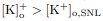, (homoclinic case).

When , v_r was chosen so that the homoclinic bifurcation occurs at the same value of applied current as in the fast subsystem of the target model. This is explained in the paragraph starting at line 178 (see Eq. 2). This criterion also allows the minimum voltage values reached during spiking to be captured reasonably well (compare the green dotted line and the purple solid line in panel e of Figure 4).

We have rewritten the paragraph starting at line 186 to clarify these aspects.

(10) Bottom page 6 - reference to Figure 3e should be 4e. Also, the text mentions the shrinkage of spike amplitude, but the figure shows that vth increases over most of the K+ range before decreasing, so a correction is needed.

We corrected the figure reference.

The maximal voltage of the limit cycles of the target model’s fast subsystem (upper purple curve in Figure 4e) increases slightly between and , by less than 1mV. It then decreases by about 27mV before the fold of limit cycles. The sigmoidal function vth () allows us to capture this substantial decrease in the QIF model. The small preceding increase is not captured. We reformulated the text to avoid confusion (see paragraph starting at line 209).

(11) Figure 4d: Why is E_K plotted here? It should be mentioned in the caption and text. More generally, the caption for Figure 4e should be expanded to mention what the purple curves are, what is the black curve for K < K_SNL, and what the other structures shown are. Finally, the text describes that theSNIC/SNL/Hom is determined by the choice of v_r relative to v_SN, so it’s not clear what is I_app,SNL in the caption - please clarify.

In conductance-based models, higher weakens the potassium concentration gradient, thereby raising E_K. The sodium and potassium reversal potentials typically bound voltage oscillations during spiking (see for example Chander and Chakravarthy, PLOS ONE, 10.1371/journal.pone.0048802, 2012), so the minimum voltage of spikes is expected to be higher when is larger. We plotted E_K in Figure 4d to show that the increase of the reset voltage v_r at larger reflects this effect in the QIF version of the model. We clarified this in the caption of Figure 4 and in the text (see paragraph starting at line 199).

Purple curves show families of limit cycles, while black curves, including the one for , show families of fixed points. The green curve shows the linear fit of v_r from panel d. All these have now been included in the legend.

In the QIF model, the onset bifurcation (SNIC, SNL, or homoclinic) is indeed determined by the choice of v_r relative to v_SN. Figure 4e shows the bifurcation diagram of the fast subsystem of the conductance-based model (Wang-Buzsáki). This is a bifurcation diagram with respect to , for a fixed value of applied current. We chose to fix I_app at its value at the SNL bifurcation, denoted I_app,SNL. I_app,SNL is near 0.22 (see Figure 3a).

(12) Eqn. (2a): Shouldn’t v_SN depend on potassium like I_SN and I_pump do? What is the formula for Ipump there? Why isn’t the RHS of (2b) dependent on v as in the original model? Please clarify.

For simplicity, we did not include a potassium dependence for v_SN in the QIF model. Instead, we set it to its value at the SNL bifurcation (Figure 4b). This is explained in the paragraph starting at line 199: “We notice that v_SN and the normal form coefficient a are relatively conserved in this interval. We fix them to their value at [K⁺]_o,SNL.”

The formula for I_pump is given in Eq. 5d. The potassium dynamics depends on the voltage via the reset rule in Eq. 3d. This allows us to capture the small increments in at each action potential in the original model (see for example Figure 6c,h). We have clarified these two points in the manuscript (see paragraph starting at line 223).

(13) Figure 3: Please indicate the criticality of the Hopf bifurcations shown.

The legend of Fig. 3 now indicates that the Hopf bifurcations are subcritical. The same clarification has been added to the following figures as well.

(14) Bottom pg. 9: Why isn’t there an I_pump term as in eqn. (6a)? Please clarify. 

You are correct, the I_pump term should be included in the equation for the averaged slow subsystem of the QIF model (see paragraph starting at line 243); it was accidentally omitted in the manuscript. Thank you for pointing this out.

(15) Top pg. 11: It’s important to reference the slow averaged dynamics here, which allows K+ to increase. Also, this first paragraph should already explain that this averaged dynamics is only relevant along the family of FS periodic orbits, not during the recovery when the FS has a branch of stable equilibria.

The averaged slow subsystem is indeed only relevant along families of limit cycles of the fast subsystem. Along families of equilibria, averaging is not necessary and the standard slow subsystem can be used. We now explicitly define this standard slow subsystem for both Wang-Buzsáki and the QIF model (see paragraphs starting at lines 241 and 628). In panels e and j of Figure 6, both systems are now represented.

In the paragraph starting at line 273, we now refer to the averaged slow subsystem to explain the overall increase of during bursts (purple curves in Fig. 6e,j), and to the standard slow subsystem to explain the decrease of during quiescent phases (black curves).

(16) Pg. 11, par 3: This is unnecessarily confusing. Please try to reword and clarify this paragraph.

We have simplified this paragraph (starting at line 293). The key point is that the reduction to the averaged slow subsystem is not valid too close to the homoclinic bifurcation.

(17) Pg. 13, end of Scenario 2: Is there any evidence this is a canard effect and not a noise effect? If so, please mention the evidence; otherwise, perhaps take this out.

What happens there appears to be a noise-induced canard effect: in the beginning of the burst, the system follows a family of stable limit cycles of the fast subsystem, i.e. a stable object. However, at some point, noise induces a transition to a portion of trajectory where the system evolves near the saddle branch, i.e. a repelling object, for a substantial amount of time. Such phenomena have been thoroughly investigated in the literature, and can also be obtained in a deterministic way; see for example Marin et al. (Physical Review E 90, 042718, 2014). Bursting traces similar to the one in Figure 7c are observed experimentally (see, for example, Figure 4c of Marin et al.), which is why we considered it worth mentioning. We have revised the paragraph starting at line 332 to clarify this point.

(18) I only see 4 curves in Figure 9a,c, but the legend has 5. Are two on top of each other? Please clarify.

Yes, the curve for = 7.21mM lies beneath the curve for = 5.21mM. This has been clarified in the figure caption.

(19) Text should note that the QIF iPRC does not develop a negative region at high K+ and high phase, as WB iPRC does.

We have updated the paragraph starting at line 409 to mention this.

(20) Pg. 16, line 4: “at the network scale” is cryptic - a more precise phrase would be preferable.

We have reformulated the sentence to clarify its meaning (see paragraph starting at line 380).

(21) Pg. 16, line 9: Reordering of words could make this clearer.

Done (see paragraph starting at line 385).

(22) Pg. 16: I am confused by line 14 because the big changes in the iPRC in Figure 9c do not align with the spike phase in Figure 9d. Please clarify what is meant here.

In the QIF model, at a given phase, the iPRC is the inverse of the slope of the voltage trace as a function of phase. Flatter slopes in Figure 9d therefore correspond to larger iPRC values in Figure 9c. This is illustrated in Figure S5. We have revised the paragraph starting at line 393 to make this point clearer.

(23) Pg. 16: Please clarify what is meant by a “delta synapse”.

By “delta synapse,” we meant a configuration in which each spike induces an instantaneous voltage jump in the postsynaptic neuron, modeled using the Dirac delta distribution. We have replaced the term “delta synapse” with “pulse-coupled,” which is more commonly used in the literature, and have added a clarification at its first occurrence in the manuscript.

(24) Discussion, line 2: Delete comma.

Done.

(25) Importantly, as noted above, the first par. needs to be rewritten since the presented method won’t work directly from data or from a target model for which most of the parameters, and hence the bifurcation diagram, are not known.

As mentioned above, we have included a new paragraph in the Discussion, starting at line 549, to clarify this point.

(26) Pg. 18: ”Originally” → ”Typically”, perhaps?

Done.

(27) Note the work of Marder et al. on temperature-related neural variability.

We thank the reviewer for this comment. We have added two relevant references from the work of Marder and colleagues addressing temperature-dependent neural variability and ionic concentrations in our manuscript (see the sentence starting on line 537).

(28) Pg. 20: Cut the ”Potassium dynamics and network models” subsection since it does not add anything substantive as written (or else expand it and include it in the subsection below).

We have expanded this paragraph and incorporated it into the subsequent subsection, as suggested by the reviewer.

(29) Finally, it’s a bit confusing that the authors refer to the potassium concentration as a slow variable yet have an instantaneous jump in this quantity at reset in their QIF model (i.e., instantaneous is VERY fast). Some explanation about this should be provided. Do they make the general assumption that ∆_K is small, for example, such that this reset reflects the slow nature of K+ evolution (i.e., during the reset period, K+ would only change slowly, and hence by a small amount)?

Yes, ∆_K is chosen to be small, to capture the behavior of the original model (compare for example panels c and h of Figure 6). As a result, in the QIF model, in the same way as in the original model, despite the fact that the dynamics of includes a fast component, on average evolves slowly. By using the averaging method, we can determine whether overall increases or decreases.

We clarified this in the manuscript, in the paragraph starting at line 243.

Reviewer #2 (Public review):

Summary:

The authors derive an integrate-and-fire model to describe the dynamics of a more complex Wang-Buzsaki model and compare the two models. A detailed discussion of bifurcation schemes in both models is convincing and allows us to evaluate the simpler model.

Strengths:

The idea is interesting, and the mathematical approach appears to be convincing. In addition, differences between the simple and original models are also discussed.

Weaknesses:

A comparison to experimental data is necessary to support the theoretical work.

As mentioned above in our answer to Reviewer 1, we demonstrate our method using as target the bifurcation diagram of a more realistic neuron model. Ideally, one would want to derive phenomenological models that capture bifurcation structures obtained from data. However, this is challenging and beyond the scope of the present study. We hope that this work encourages the development of such methods. We have revised the Introduction (see lines 52-57) and added a paragraph in the Discussion (see the paragraph starting at line 549) addressing this point.

Reviewer #2 (Recommendations for the authors):

The manuscript is well-structured; however, it appears that it has been edited with less care. Please see comments below:

(1) Page 2: “A third bifurcation, the saddle-homoclinic orbit (HOM) bifurcation,”: provide a reference for the bifurcation.

We have added a reference to the book by Izhikevich (see paragraph starting at line 63).

We have added additional references in the Introduction that we considered helpful.

(2) Page 3: “while a larger concentrations it is mediated by...”: remove “it”.

There was indeed a typo in this sentence. The intended phrasing is: “while at larger concentrations it is mediated by...”. We have corrected it accordingly (paragraph starting at line 134).

(3) Figure 2, caption: “dashed lines for unstable branches”: this is a dotted line.

Corrected to “dotted lines”. Thank you.

(4) Page 4: “is smaller than vSN (Fig. 3c),”: this figure panel does not exist, as well as the Fig.3d referred to afterwards. Please correct.

We intended to refer to Fig. 2. Figure references have been corrected. See paragraph starting at line 154.

(5) Page 6: “Fig. 3a-d shows ISN,0, vSN and a for [K]+o between 4 and 16 mM”: Fig.3c+d do not exist, please correct. Similar comment to “the absence of pump (Fig. 3e).” on the same page.

We intended to refer to Fig. 4. Figure references have been corrected (paragraphs starting at lines 199 and 209).

(6) Page 8: “(panel A)” → ”panel (a)”.

Done.

(7) Figure 4e: What is the meaning of the green dotted curve?

This curve represents the linear fit of the reset voltage v_r from panel d of Fig. 4, to show that the minimal voltage values of the limit cycles are also well captured. We have added this curve to the legend and included a brief explanation in the figure caption.